MONANOVA - Monotone regression
MONANOVA and monotone regression involve a monotonic transformation of the dependent variables. They are available in Excel using the XLSTAT software.

The MONANOVA model
Monotone regression and the MONANOVA model differ only in the fact that the explanatory variables are either quantitative or qualitative. They are based on linear regression in the first case, and on the ANOVA model in the second. These methods are based on iterative algorithms based on the ALS (alternating least squares) algorithm. Their principle is simple, it consists of alternating between a conventional estimation using linear regression or ANOVA and a monotonic transformation of the dependent variables (after searching for optimal scaling transformations).
The MONANOVA algorithm was introduced by Kruskal (1965) and the monotone regression and the works on the ALS algorithm are due to Young et al. (1976).
These methods are commonly used as part of the full profile conjoint analysis. XLSTAT-Conjoint allows applying them within a conjoint analysis (see chapter on conjoint analysis based on full profiles) as well as independently.
The monotone regression tool (MONANOVA) combines a monotonic transformation of the responses to a linear regression as a way to improve the linear regression results. It is well suited to ordinal dependent variables.
XLSTAT-Conjoint analysis software allows you to add interactions and to vary the constraints on the variables.
What is MONANOVA - Monotone Regression?
Monotone regression combines two stages: an ordinary linear regression between the explanatory variables and the response variable and a transformation step of the response variables to maximize the quality of prediction.
The algorithm is:
Run an OLS regression between the response variable Y and the explanatory variables X. We obtain the beta coefficients. Calculation of the predicted values of Y: Pred (Y) = beta * X Transformation of Y using a monotonic transformation (Kruskal, 1965) so that Pred(Y) and Y are close (using optimal scaling methods). Run an OLS Regression between Ytrans and the explanatory variables X. This gives new values for the beta. Steps 2 through 4 are repeated until the change in R² from one stage to another is smaller than the convergence criterion.
Options for MONANOVA in Excel using the XLSTAT software
You can run your MONANOVA statistical analysis either on qualitative or quantitative samples of explanatory variables. You can have several dependent variables, but they have to be quantitative.
You can also choose a level of Tolerance which prevents you from taking into account variables which might be either constant or too correlated with other ones already used in the model during your OLS regression. Moreover, you can set up a level of Interaction from 1 to 4.
You are able to choose a confidence interval level (95% by default) and define constraints on the parameters of the first and last categories of each factor, as well as on their sum by setting it to zero for example.
To stop your analysis, you can either fix a maximum number of iterations or fix a maximum value of improvement of the R2 indicator from one iteration to another. Once these values are reached, the Alternating least squares algorithm will stop.
You can manage groups of missing data by removing them, or estimating them by the mean, mode, or nearest neighbor.
Results for MONANOVA in XLSTAT
The XLSTAT MONANOVA feature provides results such as the regression model, the effects of the explanatory variable on the dependent one, and the monotonic transformation performed on the dependent variable. Of course, you can also view a table of summary statistics from the data sample that gives you the mean, mode, minimum, maximum and standard deviation of each variable. A correlation matrix is displayed, which enables you to visualize the effects of variables on each other along with some multicolinearity statistics which aim to find an interaction between multiple variables at once.
What is a correlation matrix ?
A correlation matrix is used to sum up the effects of the variables on each other. A correlation coefficient close to 1 means that there will be no difference in the variation direction of the variables. For example, they both will decrease. A correlation coefficient close to -1 means that if one decreases, the other will increase. A null correlation means that there is no interaction and the variation of each variable is completely independent.
What are multicolinearity statistics?
The displayed multcolinearity statistics are the Tolerance and the Variance Inflation Factor.
The Tolerance statistic is calculated by calculating the R2 statistic for each variable, taken as dependent with the other ones taken as explanatory, and substracting it from 1. The R2 is a statistical coefficient that indicates the percentage or explained variability of models. The closer it is to 1, the better the model.
The Variance Inflation Factor is calculated by taking 1 over the Tolerance.
What are the goodness of fit statistics?
After the summary statistics, you will be able to see the goodness of fit coefficients of the model. In a first table, the R2 statistic is displayed along with the mean squared error and the number of degrees of freedom of the model.
In a second table, other coefficients such as Wilks' Lambda also enable us to measure the significance of the model.
Another table designed to sum up its variance, like in a classic ANOVA, contains the sum of squares, mean squares as well as the degrees of freedom of the model itself, the error and of the corrected total.
Two to three tables containing the sum of squares are returned, for each type.
- The table of Type I SS values is used to visualize the influence that progressively adding explanatory variables has on the fitting of the model, as regards the sum of the squares of the errors (SSE), the mean squared error (MSE), Fisher's F, or the probability associated with Fisher's F.
- The table of Type II SS values acts in a similar way but by removing explanatory variables.
- The table of Type III SS values can be equal to the second one, but does not depend on the number of observations per cell. For a balanced design, Type II SS and Type III SS are equal.
The parameters of the model table displays the estimate of the parameters, the corresponding standard error, the Student’s t, the corresponding probability, as well as the confidence interval.
The table of standardized coefficients are used to compare the relative weights of the variables. The higher the absolute value of a coefficient, the more important the weight of the corresponding variable. When the confidence interval around standardized coefficients has value 0 (this can be easily seen on the chart of standardized coefficients), the weight of a variable in the model is not significant.
The predictions and residuals table shows, for each observation, its weight, the observed value of the dependent variable, the transformed value of the dependant variable, the model's prediction, the residuals, and the confidence intervals. Two types of confidence interval are displayed: a confidence interval around the mean (corresponding to the case where the prediction would be made for an infinite number of observations with a set of given values for the explanatory variables) and an interval around the isolated prediction (corresponding to the case of an isolated prediction for the values given for the explanatory variables). The second interval is always greater than the first, the random values being larger.
XLSTAT Charts for MONANOVA - Monotone Regression in Excel
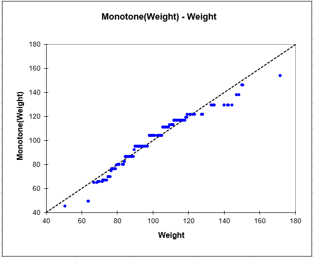
Transformation of the dependent variable chart
We can see the transformation of the dependant variable into a monotonous one.
Several examples and applications are available on our webiste which will help you set up and interpret a MANOVA analysis or similar ones according to your needs:


analyze your data with xlstat
Included in