Ordinary Least Squares regression (OLS)
Ordinary Least Squares regression (OLS), often called linear regression, is available in Excel using the XLSTAT add-on statistical software.

Ordinary Least Squares regression (OLS) is a common technique for estimating coefficients of linear regression equations which describe the relationship between one or more independent quantitative variables and a dependent variable (simple or multiple linear regression), often evaluated using r-squared. Least squares stand for the minimum squares error (SSE). Maximum likelihood and Generalized method of moments estimator are alternative approaches to OLS.
In practice, you can use linear regression in many fields:
- meteorology, if you need to predict temperature or rainfall based on external factors.
- biology, if you need to predict the number of remaining individuals in a species depending on the number of predators or life resources.
- economy, if you need to predict a company’s turnover based on the amount of sales.
- … and many more.
Statsmodels 0.15.0 and XLSTAT both offer linear regression functionalities, but they differ significantly in terms of their features, usage, and target audiences.
A bit of theory: Equations for the Ordinary Least Squares regression
The ordinary least squares formula: what is the equation of the model?
In the case of a model with p explanatory variables, the OLS regression model writes:
Y = β0 + Σj=1..p βjXj + ε
where Y is the dependent variable, β0, is the intercept of the model, X j corresponds to the jth explanatory variable of the model (j= 1 to p), and e is the random error with expectation 0 and variance σ².
In the case where there are n observations, the estimation of the predicted value of the dependent variable Y for the ith observation is given by the regression equation:
yi = β0 + Σj=1..p βjXij
Example: We want to predict the height of plants depending on the number of days they have spent in the sun, where days spent in the sun is an independent variable. Before getting exposure, they are 30 cm. A plant grows 1 mm (0.1 cm) after being exposed to the sun for a day.
- Y is the height of the plants
- X is the number of days spent in the sun
- β0 is 30 because it is the value of Y when X is 0.
- β1 is 0.1 because it is the coefficient multiplied by the number of days.
A plant being exposed 5 days to the sun has therefore an estimated height of Y = 30 + 0.1*5 = 30.5 cm.
Of course, it is not always exact, which is why we must take into account the random error ε (or the null hypothesis being tested).
Moreover, before predicting, our method must find the beta coefficients: we just start out by inputting a table containing the heights of several plants along with the number of days they have spent in the sun. If you want to find out more about the calculations, read the next paragraph.
How do ordinary least squares (OLS) work?
The OLS method aims to minimize the sum of square differences between the observed and predicted values, considering potential issues of multicollinearity.
That way, the vector β of the coefficients can be estimated by the following formula
β = (X’DX)-1 X’ Dy
with X the matrix of the explanatory variables preceded by a vector of 1s, D is a matrix with the wi weights on its diagonal, and y the vector of the n observed values of the dependent variable
The vector of the predicted values can be written as follows:
y* = Xβ=X (X’ DX)-1 X’Dy
We can even the variance σ² of the random error ε by the following formula :
σ² = 1/(W –p*) Σi=1..n wi(yi - y*i)
where p* is the number of explanatory variables to which we add 1 if the intercept is not fixed, wi is the weight of the ith observation, W is the sum of the wi weights, y the * vector of the observed values and y* the vector of predicted values
What is the intuitive explanation of the least squares method?
Intuitively speaking, the aim of the ordinary least squares method is to minimize the prediction error, between the predicted and real values. One may ask themselves why we choose to minimize the sum of squared errors instead of the sum of errors directly.
It takes into account the sum of squared errors instead of the errors as they are because sometimes they can be negative or positive and they could sum up to a nearly null value.
For example, if your real values are 2, 3, 5, 2, and 4 and your predicted values are 3, 2, 5, 1, 5, then the total error would be (3-2)+(2-3)+(5-5)+(1-2)+(5-4)=1-1+0-1+1=0 and the average error would be 0/5=0, which could lead to false conclusions.
However, if you compute the mean squared error, then you get (3-2)^2+(2-3)^2+(5-5)^2+(1-2)^2+(5-4)^2=4 and 4/5=0.8. By scaling the error back to the data and taking the square root of it, we get sqrt(0.8)=0.89, so on average, the predictions differ by 0.89 from the real value.
RUN YOUR LINEAR REGRESSION MODEL
What are the assumptions of Ordinary Least Squares (OLS)?
1) Individuals (observations) are independent. It is in general true in daily situations (the amount of rainfall does not depend on the previous day, the income does not depend on the previous month, the height of a person does not depend on the person measured just before…).
2) Variance is homogeneous. Levene's test is proposed by XLSTAT to test the equality of the error variances.
3) Residuals follow a normal distribution. XLSTAT offers several methods to test normality of residuals.
Model residuals (or errors) are the distances between data points and the fitted model. Model residuals represent the part of variability in the data the model was unable to capture. The R² statistic is the part of variability that is explained by the model, crucial in the evaluation of the null hypothesis. So the lower the residuals, the higher the R² statistic.
Homoscedasticity and independence of the error terms are key hypotheses in linear regression where it is assumed that the variances of the error terms are independent and identically distributed and normally distributed. When these assumptions are not possible to keep, a consequence is that the covariance matrix cannot be estimated using the classical formula, and the variance of the parameters corresponding to the beta coefficients of the linear model can be wrong and their confidence intervals as well.
How do I set up a linear regression model in XLSTAT?
In XLSTAT, you can easily run your ordinary least squares regression without even coding, just by data selection! You just have to select your dependent variable as well as your explanatory ones.

You can select several outcomes such as Descriptive statistics of your datasets, but also Correlations and Analysis of Variance.
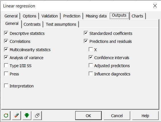
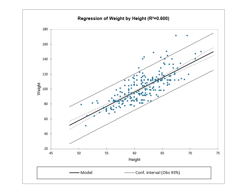
Besides statistics and the equation of the model, you can also select the charts to be displayed, such as the regression one for example. You can see all the data points and the central regression line with a confidence interval.
Predictions in OLS regression with XLSTAT
Linear regression is often used to predict outputs' values for new samples. XLSTAT enables you to characterize the quality of the model for prediction before you use the regression equation.
To go further: limitations of the Ordinary Least Squares regression
The limitations of the OLS regression come from the constraint of the inversion of the X’X matrix: it is required that the rank of the matrix is p+1, and some numerical problems may arise if the matrix is not well behaved. XLSTAT uses algorithms due to Dempster (1969) that allow circumventing these two issues: if the matrix rank equals q where q is strictly lower than p+1, some variables are removed from the model, either because they are constant or because they belong to a block of collinear variables.
What are the advantages of OLS: variable selection
An automatic selection of the variables is performed if the user selects a too high number of variables compared to the number of observations. The theoretical limit is n-1, as with greater values the X’X matrix becomes non-invertible due to multicollinearity.
The deleting of some of the variables may however not be optimal: in some cases we might not add a variable to the model because it is almost collinear to some other variables or to a block of variables, but it might be that it would be more relevant to remove a variable that is already in the model and to the new variable.
For that reason, and also in order to handle the cases where there are a lot of explanatory variables or issues like multicollinearity, other methods have been developed such as Partial Least Squares regression (PLS).
Tutorials for Ordinary Least Squares regression
Below you will find a list of examples using ordinary least squares regression analysis (OLS):


analyze your data with xlstat
Related features