Canonical Correspondence Analysis (CCA and partial CCA)
Canonical correspondence analysis investigates the links between a contingency table and a set of variables. Run CCA in Excel using the XLSTAT software.

What is Canonical Correspondence Analysis
Canonical Correspondence Analysis (CCA) has been developed to allow ecologists to relate the abundance of species to environmental variables with the assumption that relationships are gaussian. However, this method can be used in other domains. Geomarketing and demographic analyses should be able to take advantage of it.
Canonical Correspondence Analysis allows obtaining a simultaneous representation of the sites, the objects, and the variables describing the sites in two or three dimensions that are optimal for a variance criterion.
Principles of Canonical Correspondence Analysis
Let T1 be a contingency table corresponding to the counts on n sites of p objects. This table can be analyzed using Correspondence Analysis (CA) to obtain a simultaneous map of the sites and objects in two or three dimensions.
Let T2 be a table that contains the measures recorded on the same n sites of corresponding to q quantitative and/or qualitative variables.
Canonical Correspondence Analysis can be divided into two parts:
- A constrained analysis in a space which number of dimensions is equal to q. This part is the one of main interest as it corresponds to the analysis of the relation between the two tables T1 and T2.
- An unconstrained part, which corresponds to the analysis of the residuals. The number of dimensions for the unconstrained CCA is equal to min(n-1-q, p-1).
Two methods derived from Canonical Correspondence Analysis
- Partial Canonical Correspondence Analysis adds a preliminary step. The T2 table is subdivided into two groups of variables: the first group contains conditioning variables which effect we want to remove, as it is either known or without interest for the study. A Canonical Correspondence Analysis is run using these variables. A second Canonical Correspondence Analysis is run using the second group of variables which effect we want to analyze. Partial Canonical Correspondence Analysis allows you to analyze the effect of the second group of variables, after the effect of the first group has been removed.
- PLS- Canonical Correspondence Analysis: It is possible to relate discriminant PLS to Canonical Correspondence Analysis. Addinsoft is the first software editor to propose a comprehensive and effective integration between the two methods. Using a restructuring of data, a PLS step is applied to the data, either to create orthogonal PLS components that are optimally designed for the Canonical Correspondence Analysis to avoid the constraints in terms of number of variables that can be used, or to select the most influential variables before running the Canonical Correspondence Analysis. As calculations of the Canonical Correspondence Analysis step and results are identical to what is done with the classical Canonical Correspondence Analysis, users can see this approach as a selection method that identifies the variables of higher interest, either because they are selected in the model, or by looking at the chart of the VIPs. In the case of a partial Canonical Correspondence Analysis, the preliminary step is unchanged.
Results for Canonical Correspondence Analysis in XLSTAT
- Inertia: This table displays the distribution of the inertia between the constrained Canonical Correspondence Analysis and the unconstrained Canonical Correspondence Analysis.
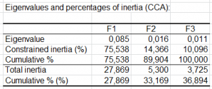
- Eigenvalues and percentages of inertia: In these tables are displayed for the Canonical Correspondence Analysis and the unconstrained Canonical Correspondence Analysis the eigenvalues, the corresponding inertia, and the corresponding percentages, either in terms of constrained inertia (or unconstrained inertia), or in terms of total inertia.
- Weighted averages: This table displays the weighted means as well the global weighted means.
- Principal coordinates and standard coordinates: The principal coordinates and standard coordinates of the sites, the objects and the variables are then displayed. These coordinates are used to produce the various charts.
- Regression coefficients: This table displays the regression coefficients of the variables in the factor space.
- Sites and objects maps:
- Sites and objects / Symmetric chart
- Site / Asymmetric
- Objects / Assymetric
- Sites
- Objects

