Sensitivity and specificity analysis

What is sensitivity and specificity analysis

Sensitivity and Specificity XLSTAT-Life function allows computing, among others, the sensitivity, specificity, odds ratio, predictive values, and likelihood ratios associated with a test or a detection method. These indices can be used to assess the performance of a test.

In medicine it can be used to evaluate the efficiency of a test used to diagnose a disease or in quality control to detect the presence of a defect in a manufactured product.

Method History

This method was first developed during World War II to develop effective means of detecting Japanese aircraft. It was then applied more generally to signal detection and medicine where it is now widely used.

Principles of Sensitivity and Specificity method

We study a phenomenon, often binary (for example, the presence or absence of a disease) and we want to develop a test to detect effectively the occurrence of a precise event (for example, the presence of the disease).

Let V be the binary or multinomial variable that describes the phenomenon for N individuals that are being followed. We note by + the individuals for which the event occurs and by ‘-those for which it does not. Let T be a test which goal is to detect if the event occurred or not. T can be a binary (presence/absence), a qualitative (for example the color), or a quantitative variable (for example a concentration). For binary or qualitative variables, let t1 be the category corresponding to the occurrence of the event of interest. For a quantitative variable, let t1 be the threshold value under or above which the event is assumed to happen.

Once the test has been applied to the N individuals, we obtain an individual/variable table in which for each individual you find if the event occurred or not, and the result of the test.

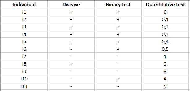
These tables can be summarized in a 2x2 contingency table:

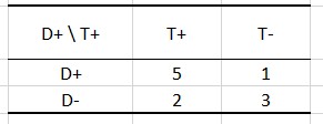
In the example above, there are 6 individuals for whom the test has detected the presence of the disease and 4 for which it has detected its absence. However, for 1 individual, diagnosis is bad because the test contends the absence of the disease while the patient is sick.

The following vocabulary is being used:

• True positive (TP): Number of cases that the test declares positive and that are truly positive.
• False positive (FP): Number of cases that the test declares positive and that in reality are negative.
• True negative (VN): Number of cases that the test declares negative and that are truly negative.
• False negative (FN): Number of cases that the test declares negative and that in reality are positive.

Indices for Sensitivity and Specificity analysis

Several indices are available in XLSTAT-Life software to evaluate the performance of a test:

• Sensitivity (equivalent to the True Positive Rate): Proportion of positive cases that are well detected by the test. In other words, the sensitivity measures how the test is effective when used on positive individuals. The test is perfect for positive individuals when sensitivity is 1, equivalent to a random draw when sensitivity is 0.5. If it is below 0.5, the test is counter-performing and it would be useful to reverse the rule so that sensitivity is higher than 0.5 (provided that this does not affect the specificity). The mathematical definition is given by: Sensitivity = TP/(TP + FN).
• Specificity (also called True Negative Rate): proportion of negative cases that are well detected by the test. In other words, specificity measures how the test is effective when used on negative individuals. The test is perfect for negative individuals when the specificity is 1, equivalent to a random draw when the specificity is 0.5. If it is below 0.5, the test is counter performing-and it would be useful to reverse the rule so that specificity is higher than 0.5 (provided that this does not affect the sensitivity). The mathematical definition is given by: Specificity = TN/(TN + FP).
• False Positive Rate (FPR): Proportion of negative cases that the test detects as positive (FPR = 1-Specificity).
• False Negative Rate (FNR): Proportion of positive cases that the test detects as negative (FNR = 1-Sensibility)
• Prevalence: relative frequency of the event of interest in the total sample (TP+FN)/N.
• Positive Predictive Value (PPV): Proportion of truly positive cases among the positive cases detected by the test. We have PPV = TP / (TP + FP), or PPV = Sensitivity x Prevalence / [(Sensitivity x Prevalence + (1-Specificity)(1-Prevalence)]. It is a fundamental value that depends on the prevalence, an index that is independent of the quality of the test.
• Negative Predictive Value (NPV): Proportion of truly negative cases among the negative cases detected by the test. We have NPV = TN / (TN + FN), or PPV = Specificity x (1 - Prevalence) / [(Specificity (1-Prevalence) + (1-Sensibility) x Prevalence]. This index depends also on the prevalence that is independent of the quality of the test.
• Positive Likelihood Ratio (LR+): This ratio indicates to which point an individual has more chances to be positive in reality when the test is telling it is positive. We have LR+ = Sensitivity / (1-Specificity). The LR+ is a positive or null value.
• Negative Likelihood Ratio (LR-): This ratio indicates to which point an individual has more chances to be negative in reality when the test is telling it is positive. We have LR- = (1-Sensitivity) / (Specificity). The LR- is a positive or null value.
• Odds ratio: The odds ratio indicates how much an individual is more likely to be positive if the test is positive, compared to cases where the test is negative. For example, an odds ratio of 2 means that the chance that the positive event occurs is twice higher if the test is positive than if it is negative. The odds ratio is a positive or null value. We have Odds ratio = TPxTN / (FPxFN).
• Relative risk: The relative risk is a ratio that measures how better the test behaves when it is a positive report than when it is negative. For example, a relative risk of 2 means that the test is twice more powerful when it is positive that when it is negative. A value close to 1 corresponds to a case of independence between the rows and columns, and to a test that performs as well when it is positive as when it is negative. Relative risk is a null or positive value given by: Relative risk = TP/(TP+FP) / (FN/(FN+TN)).

Confidence intervals for Sensitivity and Specificity analysis

For the various presented above, several methods of calculating their variance and, therefore their confidence intervals, have been proposed. There are two families: the first concerns proportions, such as sensitivity and specificity, and the second ratios, such as LR +, LR- the odds ratio and the relative risk.

For proportions, XLSTAT allows you to use the simple (Wald, 1939) or adjusted (Agresti and Coull, 1998) Wald intervals, a calculation based on the Wilson score (Wilson, 1927), possibly with a correction of continuity, or the Clopper-Pearson (1934) intervals. Agresti and Caffo recommend using the adjusted Wald interval or the Wilson score intervals.

For ratios, the variances are calculated using a single method, with or without correction of continuity.

Once the variance of the above statistics is calculated, we assume their asymptotic normality (or of their logarithm for ratios) to determine the corresponding confidence intervals. Many of the statistics are proportions and should lie between 0 and 1. If the intervals fall partly outside these limits, XLSTAT automatically corrects the bounds of the interval.

Tutorials

• Sensitivity and specificity analysis with XLSTAT-Life

Screenshots